

Economic models are really, really cool. For the small price of losing accuracy with respect to the real way of things (call it nuance), we get to feel as economists that we more or less understand why and how things happen. Our figments become formalisations.
I wanted to dip my toes into this ocean of possibilities by building my own basic model. I then draw some conclusions based on the solutions to the equations. In other words, keep reading if mixing models’ inherent flaws with the inexperience of a budding economist sounds like an interesting proposition. Suspend your disbelief, as this is going to be fun.
The body of the post will only cover the main intuition, with more information being available in the appendix.
✧✦✧
Considering my posting history, it’s only fitting that my first model be a gauge for central bank interest rates. I’ll take a different approach from the traditional IS-LM or Taylor rule route by building a model revolving around the ECB’s reaction function. This three-pronged function has been a key part of the bank’s communication ever since March 2023, and serves to better explain why the ECB takes the decisions that it does. As anticipated, it has three components:
- The inflation outlook (o)
- The dynamics of underlying inflation (u)
- The strength of monetary policy transmission (m)
In building our functions, we’ll treat each pillar as an endogenous variable. This means that their scope is defined by functions set within the model. Through the equations, each period (month) will receive its own values.
Inflation outlook (o)
Interest rate decisions today depend on inflation both today and tomorrow. In their quadrennial macroeconomic projections, the ECB reports their expected inflation values for two years into the future. For our exercise, we are interested in (i) by how much projections 12 months from now diverge from the 2% medium-term target, and (ii) the scale of revisions to the inflation outlook.
The latter means that large revisions compared to the previous projection signify important new macroeconomic developments. This should be reflected in our equations by increasing the coefficient of (i.e., importance given to) the outlook for that period.
Dynamics of underlying inflation (u)
Underlying inflation strips the noise out of inflation figures by addressing the core drivers of price changes. This variable will depend on the divergence of two important factors from the 2% inflation target.
First is the underlying inflation level, given by core inflation—headline inflation without some volatile elements. Then the actual dynamics, given by the momentum of core inflation. In essence, this measure compares seasonally adjusted inflation values between 3 months as opposed to 12 months. This gives a better understanding of the short-term direction of inflation.
The strength of monetary policy transmission (m)
The last pillar is the most abstract and thus difficult to model. In reality, monetary transmission is made up of a multitude of credit and financial market transmission indicators. Its scope in this model will be limited to a recursive function of previous periods’ monetary tightness yet to be transmitted, as well as that which has already hit the real economy.
All together
Together, they help define a desired relation for our model-implied interest rate.
Note that the strength of transmission m has a negative coefficient because greater strength requires less anticyclical interest movement. For example, good transmission when increasing interest rates means that the central bank will have to increase rates by less than if transmission was weak. Also note that the full expression of the interest equation is available in the appendix.
✧✦✧
All that’s left is seeing what cool things we can do with the equations that we built above. We’ll compare our model’s performance with actual ECB interest rate decisions since March 2023, when the reaction function entered the bank’s communication. This period features a significant hiking, holding, and cutting period—in other words, a perfect setup.
To do so, we solve the model using a deterministic historical simulation or perfect foresight solution method. In other words, we set a baseline from which we start to coincide with the interest rate, inflation and policy transmission data of our first period (note that the latter will feature interest rate decisions ever since 2022). Then we give the model the history of inflation shocks faced by the economy as the months progressed and let the endogenous reactions do their thing.
The result is the graph below. Both model-implied and actual interest rates have been smoothed to a monthly frequency. The bars decompose the contributing factors to our model’s policy function’s value for each month.
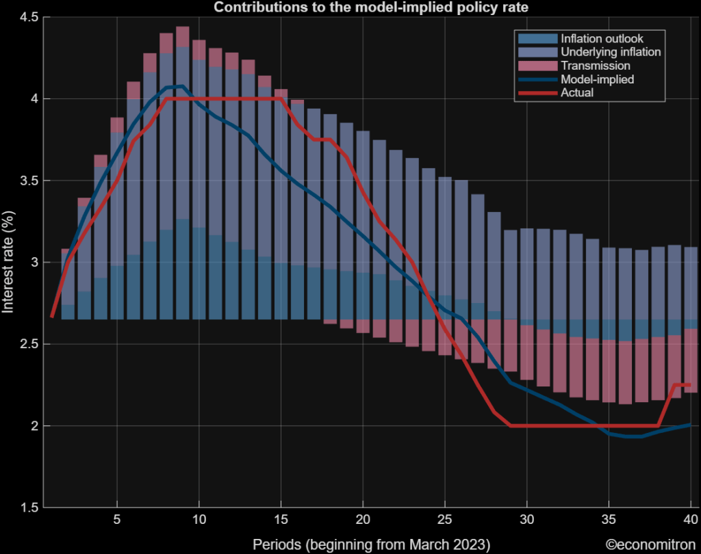
The model plots the hiking and cutting phases under baseline parametrisation, albeit leaving out the holding stage. The peak of the energy crisis is explained by an elevated inflation outlook, underlying inflationary pressures and lagging effects of loose monetary policy from Covid. This aligns closely with the historical narrative. Moreover, as upside risks to the outlook start to fade, underlying inflationary pressures in the model keep exerting headwinds on the interest rate cuts. This is something equally supported by empirical evidence.
✧✦✧
This setup leaves many interesting avenues open for future investigation. One could be to further assess the decomposition of the policy function, i.e. how the parametrisation of each pillar affects the policy rate. Another would be to use different price scenarios to guesstimate using the model the future path of interest rates, given the current energy debacle. Interest rate paths may not be certain, but the fact that they’ll feature in future posts certainly is.
Appendix
Model equations
with


Leave a Reply